Sample Splitting

This is an example using the star dataset (for more information about the dataset, please use ?star).

We start with a simple example with one outcome variable (writing scores) and one machine learning algorithm (causal forest). Then we move to incoporate multiple outcomes and compare model performances with several machine learning algorithms.

To begin, we load the dataset and specify the outcome variable and covariates to be used in the model. Next, we utilize a random forest algorithm to develop an Individualized Treatment Rule (ITR) for estimating the varied impacts of small class sizes on students’ writing scores. Since the treatment is often costly for most policy programs, we consider a case with 20% budget constraint (budget = 0.2). The model will identify the top 20% of units who benefit from the treatment most and assign them to with the treatment. We train the model through sample splitting, with the split_ratio between the train and test sets determined by the split_ratio argument. Specifically, we allocate 70% of the data to train the model, while the remaining 30% is used as testing data (split_ratio = 0.7).

library(dplyr)
library(evalITR)

load("../data/star.rda")

# specifying the outcome
outcomes <- "g3tlangss"

# specifying the treatment
treatment <- "treatment"

# specifying the data (remove other outcomes)
star_data <- star %>% dplyr::select(-c(g3treadss,g3tmathss))

# specifying the formula
user_formula <- as.formula(
  "g3tlangss ~ treatment + gender + race + birthmonth + 
  birthyear + SCHLURBN + GRDRANGE + GKENRMNT + GKFRLNCH + 
  GKBUSED + GKWHITE ")


# estimate ITR 
fit <- estimate_itr(
  treatment = treatment,
  form = user_formula,
  data = star_data,
  algorithms = c("causal_forest"),
  budget = 0.2,
  split_ratio = 0.7)
#> Evaluate ITR under sample splitting ...


# evaluate ITR 
est <- evaluate_itr(fit)
#> Cannot compute PAPDp

Thesummary() function displays the following summary statistics: (1) population average prescriptive effect PAPE; (2) population average prescriptive effect with a budget constraint PAPEp; (3) population average prescriptive effect difference with a budget constraint PAPDp. This quantity will be computed with more than 2 machine learning algorithms); (4) and area under the prescriptive effect curve AUPEC. For more information about these evaluation metrics, please refer to Imai and Li (2021); (5) Grouped Average Treatment Effects GATEs. The details of the methods for this design are given in Imai and Li (2022).

# summarize estimates
summary(est)
#> ── PAPE ────────────────────────────────────────────────────────────────────────
#>   estimate std.deviation     algorithm statistic p.value
#> 1     0.35           1.3 causal_forest      0.26    0.79
#> 
#> ── PAPEp ───────────────────────────────────────────────────────────────────────
#>   estimate std.deviation     algorithm statistic p.value
#> 1      1.8           1.3 causal_forest       1.4    0.16
#> 
#> ── PAPDp ───────────────────────────────────────────────────────────────────────
#> data frame with 0 columns and 0 rows
#> 
#> ── AUPEC ───────────────────────────────────────────────────────────────────────
#>   estimate std.deviation     algorithm statistic p.value
#> 1     0.83           1.1 causal_forest      0.79    0.43
#> 
#> ── GATE ────────────────────────────────────────────────────────────────────────
#>   estimate std.deviation     algorithm group statistic p.value  upper lower
#> 1      177           110 causal_forest     1      1.61    0.11   -3.6   357
#> 2     -143           107 causal_forest     2     -1.34    0.18 -319.0    33
#> 3      -64           107 causal_forest     3     -0.60    0.55 -240.3   112
#> 4       72           109 causal_forest     4      0.66    0.51 -107.9   252
#> 5      -32           107 causal_forest     5     -0.30    0.76 -208.1   144

We can extract estimates from the est object. The following code shows how to extract the GATE estimates for the writing score with the causal forest algorithm.

# plot GATE estimates
library(ggplot2)
summary(est)$GATE %>%
  mutate(group = forcats::as_factor(group)) %>%
  ggplot(., aes(
    x = group, y = estimate,
    ymin = lower , ymax = upper, color = algorithm)) +
  ggdist::geom_pointinterval(
    width = 0.5,
    position = position_dodge(0.5),
    interval_size_range = c(0.8, 1.5),
    fatten_point = 2.5) +  
  theme_bw() +
  theme(panel.grid = element_blank(),
        panel.background = element_blank()) +
  labs(x = "Group", y = "GATE estimate") +
  geom_hline(yintercept = 0, linetype = "dashed", color = "#4e4e4e") +
  scale_color_manual(values = c("#0072B2", "#E69F00", "#56B4E9", "#009E73", "#076f00"))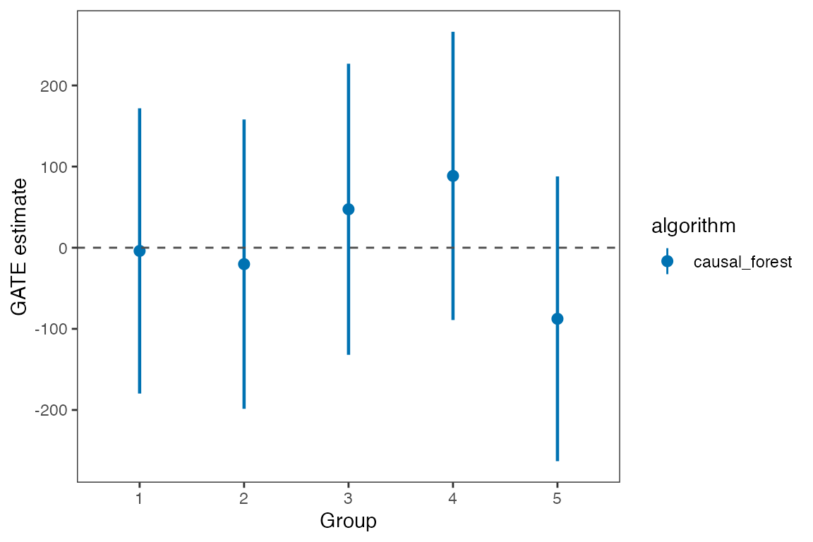

We plot the estimated Area Under the Prescriptive Effect Curve for the writing score across a range of budget constraints for causal forest.

# plot the AUPEC 
plot(est)