User Defined ITR • evalITR

Instead of using the ITRs estimated by evalITR models, we can define our own ITR and evaluate its performance using the evaluate_itr function. The function takes the following arguments: itr_function a function defined by users that returns a vector of 0 and 1, data a data frame, treatment a character string specifying the treatment variable, outcome a character string specifying the outcome variable, budget a numeric value specifying the maximum percentage of population that can be treated under the budget constraint., and tau a numeric vector specifying the unit-level continuous score for treatment assignment. We assume those that have tau<0 should not have treatment. Conditional Average Treatment Effect is one possible measure.. The function returns an object that contains the estimated GATE, ATE, and AUPEC for the user defined ITR.

# user's own ITR
my_function <- function(data){
  itr <- (data$race == 1)*1
  return(itr)
}

# evalutate ITR
user_itr <- evaluate_itr(
  itr_function = "my_function",
  data = star_data,
  treatment = treatment,
  outcome = outcomes,
  budget = 0.2,
  tau = seq(0.1, 0.9, length.out = nrow(star_data)))

# summarize estimates
summary(user_itr)
#> ── PAPE ────────────────────────────────────────────────────────────────────────
#>   estimate std.deviation   algorithm statistic p.value
#> 1    -0.43          0.69 my_function     -0.62    0.53
#> 
#> ── PAPEp ───────────────────────────────────────────────────────────────────────
#>   estimate std.deviation   algorithm statistic p.value
#> 1     0.11          0.64 my_function      0.17    0.87
#> 
#> ── PAPDp ───────────────────────────────────────────────────────────────────────
#> data frame with 0 columns and 0 rows
#> 
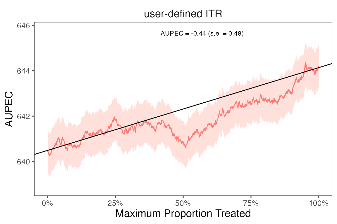
#> ── AUPEC ───────────────────────────────────────────────────────────────────────
#>   estimate std.deviation statistic p.value
#> 1    -0.44          0.48     -0.92    0.36
#> 
#> ── GATE ────────────────────────────────────────────────────────────────────────
#>   estimate std.deviation   algorithm group statistic p.value upper lower
#> 1       59            59 my_function     1      0.99   0.320   -39   156
#> 2       33            59 my_function     2      0.56   0.577   -64   130
#> 3     -153            59 my_function     3     -2.61   0.009  -250   -57
#> 4      -12            59 my_function     4     -0.20   0.838  -109    85
#> 5       92            59 my_function     5      1.56   0.119    -5   189

We can extract estimates from the est object. The following code shows how to extract the GATE estimates for the writing score with the causal forest algorithm.

# plot GATE estimates
library(ggplot2)
summary(user_itr)$GATE %>%
  mutate(group = forcats::as_factor(group)) %>%
  ggplot(., aes(
    x = group, y = estimate,
    ymin = lower , ymax = upper, color = algorithm)) +
  ggdist::geom_pointinterval(
    width = 0.5,
    position = position_dodge(0.5),
    interval_size_range = c(0.8, 1.5),
    fatten_point = 2.5) +  
  theme_bw() +
  theme(panel.grid = element_blank(),
        panel.background = element_blank()) +
  labs(x = "Group", y = "GATE estimate") +
  geom_hline(yintercept = 0, linetype = "dashed", color = "#4e4e4e") +
  scale_color_manual(values = c("#0072B2", "#E69F00", "#56B4E9", "#009E73", "#076f00"))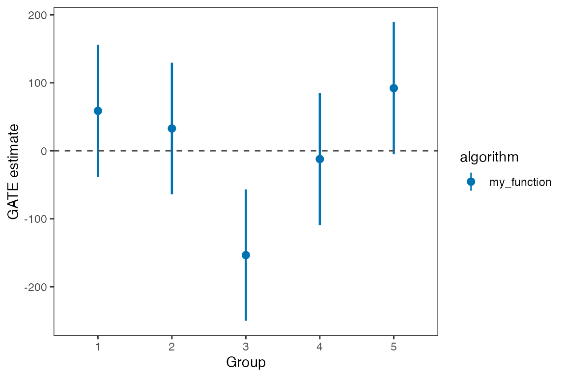

We plot the estimated Area Under the Prescriptive Effect Curve (AUPEC) for the writing score across a range of budget constraints for user defined ITR.

# plot the AUPEC 
plot(user_itr)